Logistic Map and Lyapunov Exponent

Lyapunov Exponent for the Speading of Two Close Points on a Logistic Map

LogisticMap is a C# Windows application that I developed for homework in my Statistical Mechanics class.  The application plots the spread between two points on a logistic map and calculates the Lyapunov exponent for the spreading.  LogisticMap is a solution to Exercise 5.9 in Dr. James Sethna’s Statistical Mechanics: Entropy, Order Parameters, and Complexity.

You can get the LogisticMap application and its source code on GitHub.

Here’s some background on the logistic map, chaos, and the Lyapunov exponent.  In the application, we are evaluating the following function:

f(x) = 4μx(1-x)

This function is called a logistic map because it takes a point between 0 and 1 and returns a different point that is also between 0 and 1.  It maps the unit interval (0,1) into itself.  We can think about the trajectory of an initial point, x0, on the map as being the successive results of plugging the previous result back into the function: f(x0), f(f(x0)), f(f(f(x0))), …

Trajectories on the Logistic Map (μ = 0.9)

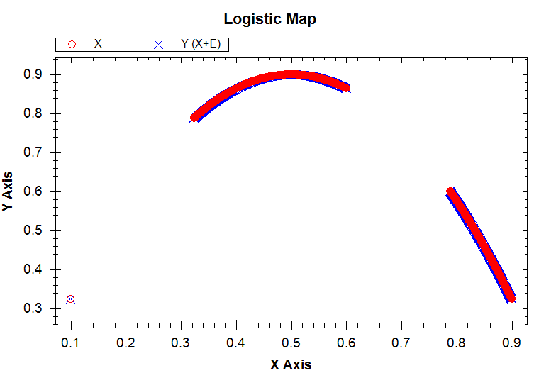
The trajectory depends on the value of the constant μ.  When μ = 0 obviously all trajectories will immediately converge to 0.  When μ = 0.5 all trajectories converge on 0.5 but not immediately. When μ = 0.9 the trajectories do not converge on one value, but instead wind up within a certain range of values (roughly between 0.3 and 0.6 and between 0.8 and 0.9).

Trajectories on the Logistic Map (μ = 1)

Now when μ = 1, the trajectories do not converge on one value and their range of values is still between 0 and 1, the same range of values that we chose for the initial point.  As Sethna states, “for μ = 1, it precisely folds the unit interval in half, and stretches it (non-uniformly) to cover the original domain”.  Furthermore, two very close initial points will have dramatically different trajectories.  This sensitive dependence on the initial point is what makes the logistic map with μ = 1 a chaotic system.

It turns out that the separation between the trajectories of the two initial points grows exponentially at a rate which is called the Lyapunov exponent.  This exponential drifting eventually stops because the two trajectories are still pegged between 0 and 1, so there is a limit to how far apart they can be.  At this point, the distance of their separation will fluctuate randomly.

If you would like to compute the Lyapunov exponent for a chaotic system, try using the following values:

• X: 0.9 (X can be any number between 0 and 1, but not 0, 0.5, or 1)
• E: 0.00000001 (E is the small difference between the two initial points, x0 and x0+E, so it should be very small)
• N: 50 (N is the number of computed trajectory points, so it should be reasonably large enough that the exponential spreading of the two points can be computed)
• Mu: 1 (this is what makes the logistic map a chaotic system)